Deep Learning - ANN - Artificial Neural Network - Optimizer Tutorial
Optimizers are algorithms or methods used to change the attributes of your neural network such as weights and learning rate in order to reduce the losses. Optimizers help to get results faster.
Different types of optimizer technique is -
- Gradient Descent – Batch, Stochastic and Mini-Batch
We already have optimizer techniques like gradient descent. then why it is needed for more optimizer techniques the reason is-
1] To find the right learning rate
2] The solution is a learning rate schedule, but the problem with a learning schedule is we need a predefined schedule before training, which means it does not depend on training.
3] If there are two weight parameters w1 and w2, then we can’t define the different learning parameters for different weight - restrictions.
4] Problem of multiple local minima - There are chances to get stuck in local minima rather than global minima.
5] Problem of saddle point
This is the reason why we need more optimizer techniques. which are given below-
- Momentum
- Adagrad
- NAG
- RMSProp
- Adam
before this we need to learn EWMA - exponentially weighted moving average
EWMA – exponentially weighted moving average
EWMA is a technique using which we find hidden trends in time-series based data.
The moving average is designed such that older observations are given lower weights. The weights fall exponentially as the data point gets older – hence the name is exponentially weighted.
It is used in time series forecasting, financial forecasting, signal processing, and deep learning optimizer.
Formula -
Vt = ßVt-1 + (1-ß)Øt
Vt – Exponentially weighted moving average at a particular time t
ß(beta) – constant between 0 and 1. If beta = 0.5, then
day = \(\frac{1}{1-\beta}\)= \(\frac{1}{1-0.5}\)= 2 days.
In this case, EWMA will act as a normal average of the previous 2 days.
Vt-1 - Exponentially weighted moving average at a particular time t -1
Øt – Current time instance data
| index | temp(Ø) |
| D1 | 25 |
| D2 | 13 |
| D3 | 17 |
| D4 | 31 |
| D5 | 43 |
Let ß(beta) = 0.9
V0 = 0 then V0 = Ø0
V1 = 0.9 x V0 + 0.1 x 13 = 1.3
V2 = 0.9 x 1.3 + 0.1 x 17 = 2.87
Mathematical Intuition -
Vt = ßVt-1 + (1-ß)Øt
V0 = 0
V1 = (1-ß)Ø1
V2 = ßV1 + (1-ß)Ø2 = ß(1 - ß)Ø1 + (1-ß)Ø2
V3 = ßV2 + (1-ß)Ø3 = ß2(1 - ß)Ø2 + (1-ßb)Ø3
V4 = ßV3 + (1-ß)Ø4 = ß3(1 - ß)Ø1 + ß2(1 - ß)Ø2 + ß(1-ß)Ø3 + (1-ß)Ø4 = (1 - ß)[ ß3Ø1 + ß2Ø2 + ßØ3 + Ø4 ]
ß3 is multiplying by Ø1, ß2 is multiplying by Ø2 and ß is multiplying by Ø3, but ß value lies between 0 and 1.
Such that older observations are given lower weights start from Ø1, Ø2 and Ø3
ß3 < ß2 < ß
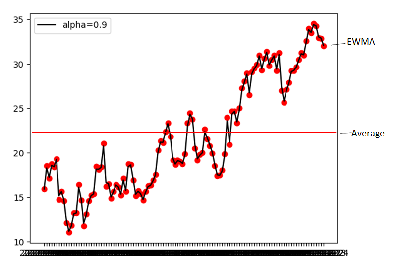
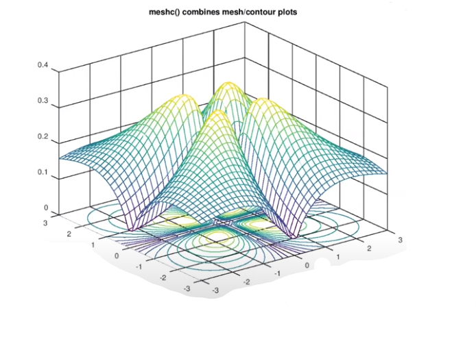
Exponetially Weighted Moving Average
For different beta, if the beta value is high, then the day will also be high, such that many old/past points will be given less weight as compared to new data points.
Understanding Graph-
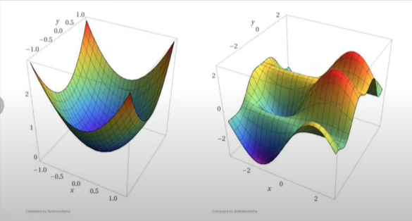
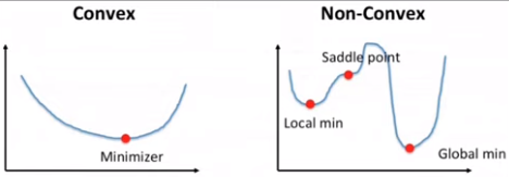
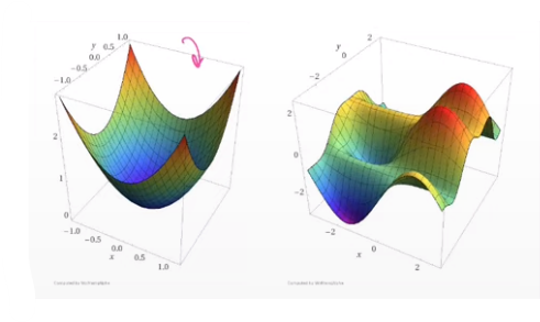
Convex Vs Non-Convex Optimization
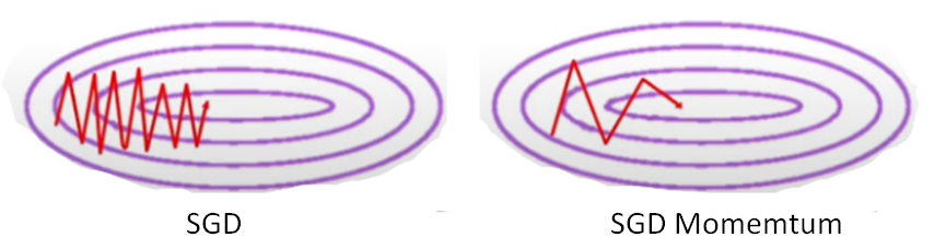
SGD with Momentum | Optimizers in Deep Learning
The problem faced by Non-convex optimization is
1] High Curvature
2] Consistent Gradient – slope change slowly
3] Noisy Gradient – Local minima
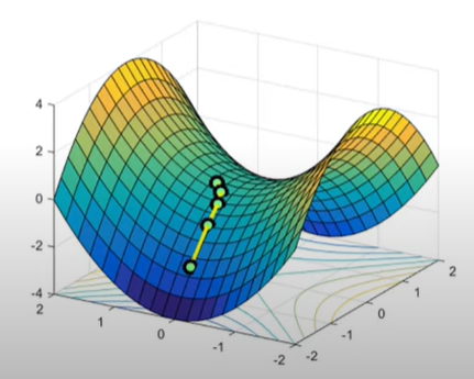
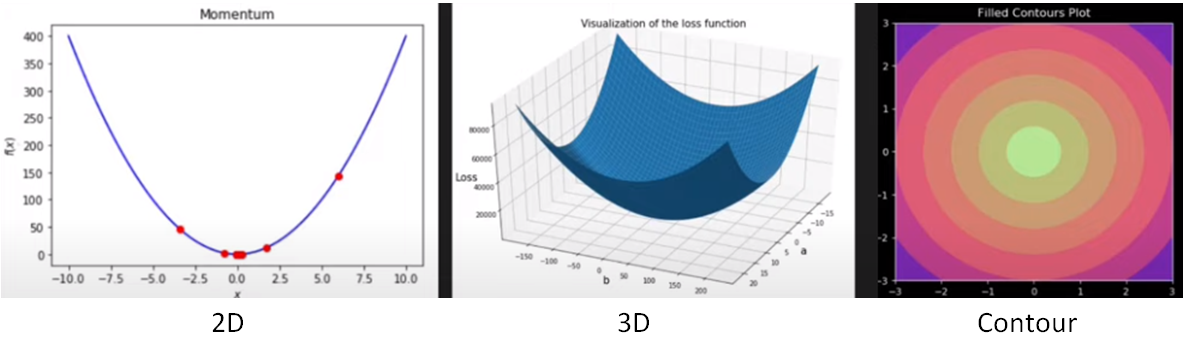
Momentum will solve the below problem-
SGD with momentum is a method that helps accelerate gradient vectors in the right directions based on previous gradients, thus leading to faster converging.
Momentum with SGD is faster than normal SGD and batch gradient descent.
Real-time example - suppose we have to reach the restaurant, the direction we don’t know, and on the road, four people provide the same direction for the restaurant, then we are 100% confident that we are reaching toward right direction and we will increase our speed.
If all four of them provide a different direction. then obviously we are 0% confident about reaching the hotel and we will decrease our speed.
How the momentum optimization work?
Wt+1 = Wt - \(\eta\lambda\)Wt
V → Velocity
Wt+1 = Wt - Vt
Vt = ß x Vt-1 + \(\eta \bigtriangledown\)Wt → History of velocity you are using it as past velocity. Due to this, it provides acceleration.
0<ß<1
When beta ß is 0, momentum will act as a normal SGD i.e Vt = Vt-1 + \(\eta \bigtriangledown\)Wt
NAG – Nesterov Accelerated Gradient
Momentum may be a good method but if the momentum is too high the algorithm may miss the local minima and may continue to rise up. So, to resolve this issue the NAG algorithm was developed.
NAG is a process of implementing momentum, but there is one improvement to reduce the oscillation.
That improvement is -
In Momentum, the jump to the next step will depend simultaneously both on the history of velocity and gradient at that point.
While in NAG, the jump to the next step will first depend on the history of velocity(momentum) till it reaches a look-ahead point, and on the next point(look ahead point), it will calculate the gradient at that point and on the basis of that it will make next jump.
Wla = Wt - ßVt-1
Vt = ßVt-1 + \(\eta \bigtriangledown\)Wla
Vt = (Wt - Wla) + \(\eta \bigtriangledown\)Wla
Wt+1 = Wt - Vt
Disadvantage – gradient descent can stuck in local minima, because of a reduction in oscillation.
Keras Implementation-
tf.keras.optimizers.SGD(
learning_rate=0.01, momentum=0.0, nestrov=False, name="SGD", **kwargs
)
For SGD – momentum = 0.0 and Nesterov = false
For momentum – momentum= any constant value (e.g 0.9 ), Nesterov = false
For Nesterov – momentum= any constant value (e.g 0.9 ), Nesterov = true
AdaGrad Optimization
Adaptive Gradient or Adagrad is used when we have sparse data.
Adagrad is an optimizer with parameter-specific learning rates, which are adapted relative to how frequently a learning rate gets updated during training. The more updates a learning rate receives, the smaller the updates.
If the gradient/slope is big then the learning rate is small and then the resultant update will also be smaller.
If the gradient/slope is smaller then the learning rate is big and then the resultant update will also be smaller.
In short, in Adagrad for different parameters, we set different learning rates.
Formula-
Wt+1 = Wt - \(\frac{\eta\bigtriangledown W_t}{\sqrt{V_t +\epsilon}}\)
Vt = Vt-1 + \({(\bigtriangledown W_t)}^2\)
where Vt is past gradient squared sum
epsilon - a small number so that the denominator value does not become zero.
Vt - Current magnitude = past magnitude + gradient2
When to use Adagrad?
1] When input features scale differently
2] When the feature is sparse(contains 0 value)
the sparse feature will create an elongated bowl problem.
In Elongated, the Slope will change on the 1st axis and remain constant on the 2nd axis.
Disadvantage-
Due to this AdaGrad is not used in neural networks -
It does not converge totally to minima, it will reach near minima after using a large no. of epoch.
the reason is as the no. of epoch increases the Vt value also increases and the learning rate decreases. due to which the update is so small and doesn’t converge to global minima.
RMSProp
Root mean square propagation - This optimization technique is an improvement of AdaGrad
The RMSprop optimizer is similar to the gradient descent algorithm with momentum. The RMSprop optimizer restricts the oscillations in the vertical direction. Therefore, we can increase our learning rate and our algorithm could take larger steps in the horizontal direction converging faster.
It will solve the problem of AdaGrad i.e. in AdaGrad it reaches global minima but it doesn’t get converge to global minima.
Formula-
Vt = ßVt-1 + (1 - ß) ( Wt)2
Wt+1 = Wt - \(\frac{\eta\bigtriangledown W_t}{\sqrt{V_t +\epsilon}}\)
where ß = 0.95
In this, we are giving more weightage to recent points than old values.
No Disadvantage
Adam Optimizer
Adaptive Moment Estimation - It is the most popular optimization technique
Adam is a replacement optimization algorithm for stochastic gradient descent for training deep learning models. Adam combines the best properties of the AdaGrad and RMSProp algorithms to provide an optimization algorithm that can handle sparse gradients on noisy problems
Formula-
Wt+1 = Wt - \(\frac{\eta\times M_t}{\sqrt{V_t +\epsilon}}\)
where
Mt = ß1Mt-1 + (1 - ß1) \(\bigtriangledown W_t\) → momentum
Vt = ß2Mt-1 + (1 - ß2)(\(\bigtriangledown W_t\))2→ Adagrad