Deep Learning - ANN - Artificial Neural Network - Perceptron Tutorial
A Perceptron is a neural network unit that does certain computations to detect features or business intelligence in the input data. It is a function that maps its input “x” which is multiplied by the learned weight coefficient, and generates an output value f(x).
Perceptron is a linear Machine Learning algorithm used for supervised learning for various binary classifiers.
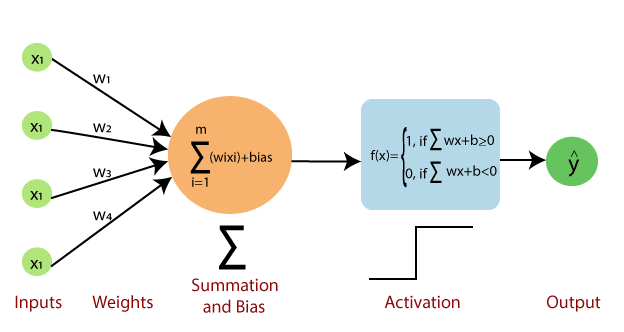
In Machine Learning, Perceptron is considered a single-layer neural network that consists of four main parameters named input values (Input nodes), weights and Bias, summation, and an activation function. The perceptron model begins with the multiplication of all input values and their weights, then adds these values together with bias to create the weighted summation and bias. Then this weighted summation and bias is applied to the activation function 'f' to obtain the desired output. This activation function is also known as the step function and is represented by 'f'.
This step function or Activation function plays a vital role in ensuring that output is mapped between required values (0,1) or (-1,1). It is important to note that the weight of input is indicative of the strength of a node. Similarly, an input's bias value gives the ability to shift the activation function curve up or down.
Weight will tell feature importance. It will tell us which feature or input is more important on the basis of weight.
Neuron VS Perceptron
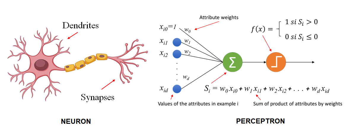
There are many similarities, but some differences also i.e.-
Similarity-
- Dendrites act as an input.
- The nucleus acts as a summation and activation function
- Axon acts as an output
- The group of neurons will make the nervous system, similarly, the group of perceptron makes multilayer perceptron.
Difference
- The neuron is more complex than the perceptron
- The processing step is simple in perceptron
- Neuron is Neuroplasticity
Perceptron is a line in 2D, a plane in 3D, a hyperplane in 4D, and soon through which we can create two regions. Hence, known as a binary classifier.
Z = W1X1 + W2X2 + b ----- 2D
Z = W1X1 + W2X2 + W3X3 + b ----- 3D
Which is similar to line equation Ax + By + C = 0
In Non-Linear Datasets perceptron will fail. Perceptron will only work well in Linear Datasets.
Practical Link - Perceptron - Demo
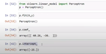
Perceptron Trick
The line that separates data in perceptron will not be in the form of y=mx+b (Linear Regression). It will be in the form of Ax+By+c=0 (Logistic Regression - General form). Our main objective is to find the value of A, B, and C to classify both the class. This is done with the help of the perceptron trick.
The perceptron trick starts by randomly assigning some values to the weights and biases. The algorithm then goes through each object and checks if it is classified correctly based on the current weights and biases. It will correctly classify itself until convergence or the end of the loop(epoch) and provide optimal weights for the input to make correct binary classifications, typically separating two classes.
How To Label Region? i.e. how to identify the positive and negative region
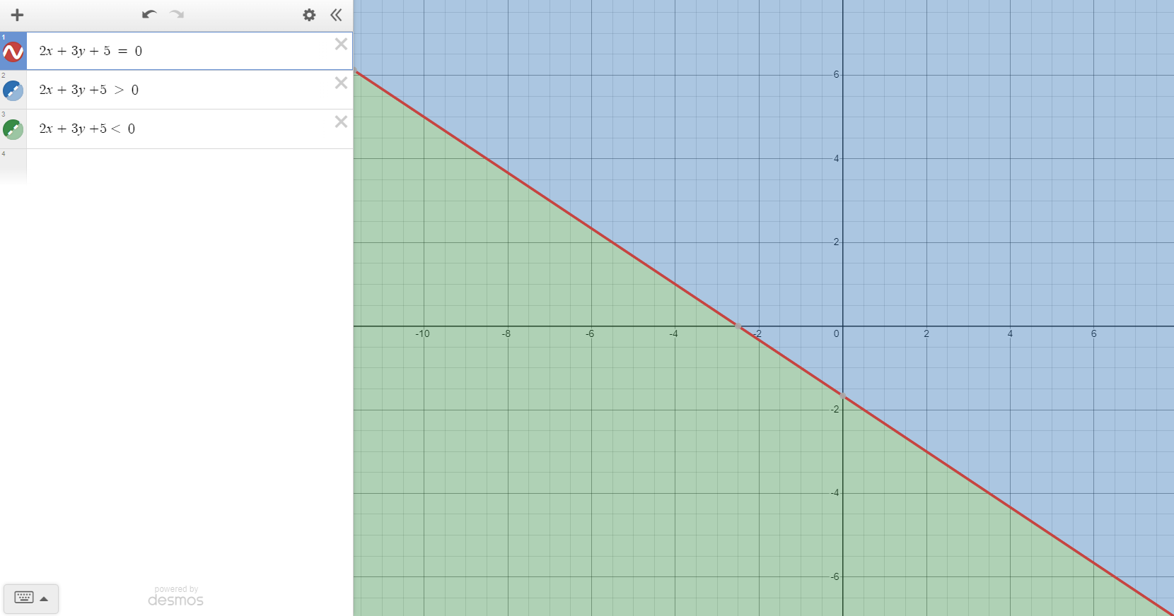
Suppose we take a Random Line with equation 2x + 3y + 5 = 0
and we have to identify positive and negative regions then 2x + 3y + 5 > 0 is positive region and 2x + 3y + 5 < 0 is negative region
Practical - Using Desmos Calculator
Transformation
Suppose there are 2 point x(5,2) Negative Point in the Positive Region and y(-3,-2) Positive Point in the Negative Region with respect to a line 2x + 3y + 5 = 0
Calculation -
Perceptron trick says to add 1 in point i.e. x(5,2,1) and y(-3,-2,1)
For the negative point x(5,2,1) in the positive region, we will subtract the value from the line equation i.e.
2 3 5
-[5 2 1]
= -3x + 1y + 4 = 0
Now x(5,2) Negative Point is in the Negative Region with respect to a line -3x + 1y + 4 = 0
For the positive point y(-3,-2,1) in the negative region, we will add the value from the line equation i.e.
2 3 5
+[-3 -2 1]
= -1x + 1y + 6 = 0
Now x(-3,-2) Positive Point is in the Positive Region with respect to a line -3x + 1y + 4 = 0
Practical - Using Desmos Calculator
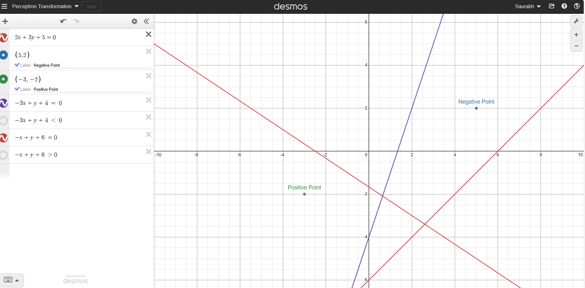
But in machine learning, we never apply transformation in a single step(exponential step) i.e. 1st line was 2x + 3y + 5, then it exponentially becomes -3x + 1y + 4. It transforms slowly based on the learning rate(mostly it is 0.01 or 0.1).
Algorithm
Line Equation-
Ax + By + c = 0
we can also write this in the below form-
W0 + W1X1 + W2X2 = 0
W0 = c (bias), W1 = A, W2 = B
let's take X0 = 1, Then the equation becomes-
W0X0 + W1X1 + W2X2 = 0
∑2i=0WiXi=0
if W0 + W1X1 + W2X2 > = 0 ----> 1, then it lies in the positive region
if W0 + W1X1 + W2X2 < 0 -----> 0, then it lies in the negative region
epoch - no. of time loop will run
n - learning rate(mostly it is 0.1 or 0.01)
for i in range(epochs):
randomly select a student
if Xi belongs to N(Negative Point) and ∑2i=0WiXi>=0 (But Point Lies in Positive Region)
Wnew = Wold - nXi (Then update the Wold Value to bring Negative Point back in Negative Region)
if Xi belongs to P(Positive Point) and ∑2i=0WiXi<0 (But Point Lies in Negative Region)
Wnew = Wold + nXi (Then update the Wold Value to bring Positive Point back in Positive Region)
Simplified Algorithm-
| Yi (Actual Placement) | Y'i ( Model Placement) | Yi - Y'i | Result |
| 1 | 1 | 0 | Wn = Wo |
| 0 | 0 | 0 | Wn = Wo |
| 1 | 0 | 1 | Wn = Wo + nXi |
| 0 | 1 | -1 | Wn = Wo - nXi |
for i in range(epochs):
randomly select a student
Wn = Wo + n(Yi - Y'i) Xi
Practical Link - Perceptron Trick