Deep Learning - ANN - Artificial Neural Network - Gradient Descent | Batch, Stochastics, Mini Batch Tutorial
Gradient Descent is one of the most popular algorithms to perform optimization and by far the most common way to optimize neural networks.
Gradient Descent is a way to minimize an objective function J(Ø) parameterized by a model's parameters θ∈Rdd by updating the parameters in the opposite direction of the gradient of the objective function ∇θJ(θ) wrt to the parameters.
The learning rate η determines the size of the steps we take to reach a (local) minimum.
In other words, we follow the direction of the slope of the surface created by the objective function downhill until we reach a valley.
There are three variants types of Gradient Descent-, which differ in how much data we use to compute the gradient of the objective function.
Depending on the amount of data, we make a trade-off between the accuracy of the parameter update and the time it takes to perform an update.
- Batch Gradient Descent ( Vanilla GD )
In Batch Gradient Descent, you can take the entire dataset and then make an update using the dot product in one shot.
If the epoch is 5 then the weight will get updated 5 times.
Algorithm-
for i in range(nb_epochs):
params_grad = evaluate_gradient(loss_function, data, params)
params = params - learning_rate * params_grad
- Stochastic Gradient Descent
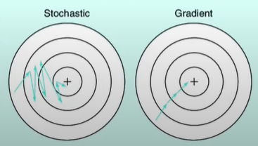
In Stochastic Gradient Descent, for each epoch, you will first shuffle the data point to get random and then update each shuffled data point one by one.
If the epoch is 5 and there is 50 data/row, then the weight will get updated 500 times.
Algorithm-
for i range(nb_epochs):
np.random.shuffle(data)
for example in data:
params_grad = evaluate_gradient(loss_function, example, params)
params = params - learning_rate * params_grad
Simplification -
epoch = 10
for i range(10):
->shuffle data x
for i in range(x.shape[0]):
-> calculate y_hat using forward propagation
-> calculate loss
-> update w,b using Wn = Wo - ηδLδW
average loss print for the epoch
- Mini Batch Gradient Descent
Mini-Batch Gradient Descent is a Combination Of Both Batch and Stochastic Gradient Descent, for each epoch, you will first shuffle the data point to get a random point then will create a mini-batch of that random data point, and then make an update of each batch using the dot product.
If there is 320 row that makes 10 batches of 32 row each(batch size). These 10 batches will be mini-batch
Algorithm-
for i range(nb_epochs):
np.random.shuffle(data)
for batch in get_batches(data, batch_size = 32)
params_grad = evaluate_gradient(loss_function, batch, params)
params = params - learning_rate * params_grad
No. of batch = No of datapoint/batch_size
In Neural Network, you have to define batch size in the model.fit() after compile(), such as if batch_size = 320, i.e. it is equal to no. of the row then it is batch gradient descent.
If batch_size = 1, then it is a stochastic gradient descent
If batch_size = 32, then each batch is of 32 sizes, and the total no. of the batch will be 320/32 i.e 10 batch
Which is faster(given the same no. of epochs)?
Batch gradient descent is fast as compared to Stochastic for the same no. of epoch.
e.g. Batch GD will take 2 sec to complete, while Stochastic GD will take 18 sec to complete for the same no. of epoch.
Batch GD > Mini Batch GD > Stochastic GD
Batch Vs Stochastic Gradient Descent Practical
Which is faster to converge(given the same no. of epochs)?
For same no. of epoch Stochastic will reach a faster point of convergence than batch.
e.g. for 10 epochs, stochastic will reach an accuracy of 98%, while batch will reach an accuracy of 60%.
Batch GD < Mini Batch GD < Stochastic GD
Stochastic Gradient Descent

Advantage-
Help the algorithm to move out of local minima and converge toward global minima because of spikiness.
Disadvantage-
Will not reach to exact solution, it will reach toward approximate solution.
Vectorization
In batch GD we have not used a loop as we have used in stochastic. instead, we used the dot product of datapoint, which is a vectorization.
The dot product is the smart replacement of a loop, which is faster than a loop.
Hence, batch GD is faster than stochastic GD
A disadvantage of vectorization-
But if there is 10cr data in the dataset then it will not work, because you have to load 10 cr data at a time in memory(RAM). It is faster for small data.
Which batch size is provided in multiple of 2 i.e. 2, 4, 8, 32, 64?
RAM is designed to handle binary values more effectively and we use batch size in multiple of 2 for better optimization technique.