Deep Learning - ANN - Artificial Neural Network - Backward Propagation Tutorial
What is BackPropagation?
It is an algorithm to train neural networks. It is the method of fine-tuning the weights of a neural network based on the error rate obtained in the previous epoch (i.e., iteration).
Backpropagation, short for "backward propagation of errors," is an algorithm for supervised learning of artificial neural networks using gradient descent. Given an artificial neural network and an error function, the method calculates the gradient of the error function with respect to the neural network's weights using the chain rule.
Prerequisite-
- Gradient Descent
- Forward Propagation
Let's take a small example-
Step 0] Initialize w and b with random values i.e w = 1, b = 0
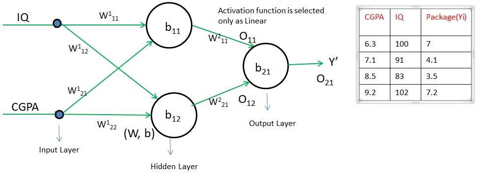
Step 1] Select any point(row from the student table). Let say CGPA = 6.3 and IQ = 100
Step 2] Predict(LPA) using forward propagation.
Let's say the predicted value is 18 and the actual value is 7. which means there is an error, it is because the value of w and b is incorrect(random)
Step 3] Choose a loss function to reduce error. We will select MSE since it is a regression case i.e. L = (Y – Y’)2 = (7 – 18)2 = 121 is the error for the 1st student.
Based on the error rate we have to adjust L’ (we can’t change L as it is actual data). To change L’ we need to adjust w and b. So the error will be minimal.
Y’ i.e O21 = W211 O11 + W221 O12 + b21
O11 = W111 IQ + W121 CGPA + b11
O12 = W112 IQ + W122 CGPA + b12
As we are going in backward direction i.e
from O21 to ‘O11 and O12 ‘ and
from (O11 to ‘W111 , W121 and b11’ and O12 to ‘W112, W122 and b12’) respectively
And there we need to make changes in w and b to reduce loss. Therefore it is called BackPropagation.
Step 4] Weight and bias need to be updated based on Gradient Descent.
Wnew=Wold−ηδLδWold
bnew=bold−ηδLδbold
As O21 depend on W211, W221, b21, O11 and O12
Therefore to update O21, we need to update W211 as, W211new=W211old−ηδLδW211to update W221 as W221new=W221old−ηδLδW221 and to update b21 a b21new=b21old−ηδLδb21
we already have Wold = 1 taken in step 0] η−value is 0.01 and we only need to find δLδW211 i.e derivative of loss with respect to weight
In the above image, there is 9 weight and bias. Hence, we need to calculate the derivative of Loss with respect to each weight and bias using the chain rule of differentiation.
[δLδW211,δLδW221,δLδb21],[δLδW111,δLδW121,δLδb11],[δLδW112,δLδW122,δLδb12]
what is dy/dy - when we make any changes in x, then how much amount of changes will happen in y
Let's try to find out the derivative of L with respect to W211 -
δLδW211=δLδY′×δY′δW211 - Chain rule of differentiation(i.e on changing W211 how much Y' will change and on changing Y' how much L will change)
δLδY′=δ(Y−Y′)2δY′=−2(Y−Y′)
δY′δW211=δ[O11W211+O12W221+b21]δW211=O11
δLδW211=−2(Y−Y′)O11
Let's try to find out the derivative of L with respect to W221 -
δLδW221=δLδY′×δY′δW221
δLδY′=δ(Y−Y′)2δY′=−2(Y−Y′)
δY′δW221=δ[O11W211+O12W221+b21]δW221=O12
δLδW221=−2(Y−Y′)O12
Let's try to find out the derivative of L with respect to b21 -
δLδb21=δLδY′×δY′δb21
δLδY′=δ(Y−Y′)2δY′=−2(Y−Y′)
δY′δb21=δ[O11W211+O12W221+b21]δb21=1
δLδb21=−2(Y−Y′)
Similarly, we can find other remaining 6 derivatives like this-
δLδW111=δLδY′×δY′δO11×δO11δW111
δLδW121=δLδY′×δY′δO11×δO11δW121
δLδb11=δLδY′×δY′δO11×δO11δb11
δLδW112=δLδY′×δY′δO12×δO12δW112
δLδW122=δLδY′×δY′δO12×δO12δW122
δLδb12=δLδY′×δY′δO12×δO12δb12
δY′δO11=δ[W211O11+W221O21+b21]δO11=W211
δY′δO12=δ[W211O11+W221O21+b21]δO12=W221
δO11δW111=δ[IQ.W111+CGPA.W121+b11]δW111=IQ let's say it is a Xi1
δO11δW121 let's say it is a Xi2
δO11δb21 = 1
δO11δW112=δ[IQ.W112+CGPA.W122+b12]δW112=IQ let's say it is a Xi1
δO12δW122 let's say it is a Xi2
δO12δb12 = 1
Therefore,
δLδW111=δLδY′×δY′δO11×δO11δW111 = -2(Y - Y') W211 Xi1
δLδW121=δLδY′×δY′δO11×δO11δW121 = -2(Y - Y') W211 Xi2
δLδb11=δLδY′×δY′δO11×δO11δb11 = -2(Y - Y') W211
δLδW112=δLδY′×δY′δO12×δO12δW112 = -2(Y - Y') W221 Xi1
δLδW122=δLδY′×δY′δO12×δO12δW122 = -2(Y - Y') W221 Xi2
δLδb12=δLδY′×δY′δO12×δO12δb12 = -2(Y - Y') W221
Summarizing Back Propagation Algorithm
epochs = 5
for i in range(epochs):
for j in range(X, Shape[0]):
-> Select 1 row(random)
-> Predict using forward propagation
-> Calculate loss using loss function - MSE
-> Update weights and bias using Gradient Descent
Wnew=Wold−ηδLδWold
-> Calculate the average loss for the epoch
δLδW221 = -2(Y - Y') O11
δLδW221 = -2(Y - Y') O12
δLδb21 = -2(Y - Y')
δLδW111 = -2(Y - Y') W211 Xi1
δLδW121 = -2(Y - Y') W211 Xi2
δLδb11 = -2(Y - Y') W211
δLδW112 = -2(Y - Y') W221 Xi1
δLδW122 = -2(Y - Y') W221 Xi2
δLδb12 = -2(Y - Y') W221
BackPropagation Regression Practical
Classification Example
We will use the Activation Function as the Sigmoid Function and the loss function as Binary Cross Entropy. Rest all process will be same as Regression
BackPropagation Classification Practical
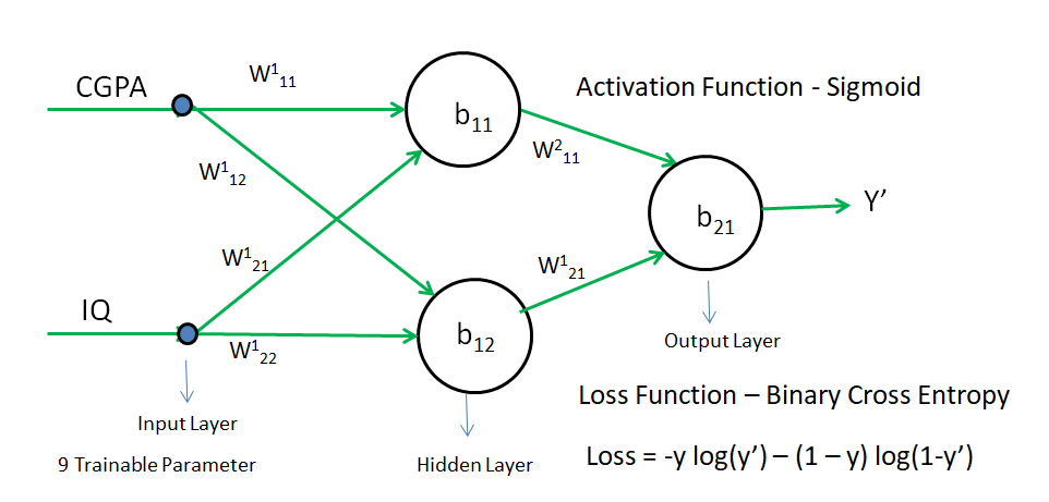
Z = W111 x CGPA + W121 x IQ + b11
Addition step in case of classification - we need to pass the Z in sigma(sigmoid function) i.e σ(Z)=O11 to get the final Output
In the above image, there is 9 weight and bias. Hence, we need to calculate the derivative of Loss with respect to each weight and bias using the chain rule of differentiation.
[δLδW211,δLδW221,δLδb21],[δLδW111,δLδW121,δLδb11],[δLδW112,δLδW122,δLδb12]
what is dy/dy - when we make any changes in x, then how much amount of changes will happen in y
L = -y log(y') - (1 - y) log(1 - y')
Let's try to find out the derivative of L with respect to W211 -
δLδW211=δLδY′×δY′δZ×δZδW211 - Chain rule of differentiation(i.e on changing W211 how much Z will change and on changing Z how much Y' will change and on changing Y' how much L will change)
δLδY′=δ[-y log(y') - (1-y) log(1-y)]δY′
=−yy′+1−y1−y′=−y(1−y′)+y′(1−y)y′(1−y′)
=−y+yy′+y′−yy′y′(1−y′)=−(y−y′)y′(1−y′)
δY′δZ=δ(σ(Z))δZ=σ(Z)[1−σ(Z)]=Y′(1−Y′)
δLδY′×δY′δZ=−(Y−Y′)Y′(1−Y′)×Y′(1−Y′)=−(Y−Y′)
δZδW211=δ(W211O11+W221O12+b21)δW211=O11
δLδW211=δLδY′×δY′δZ×δZδW211=−(Y−Y′)O11
Let's try to find out the derivative of L with respect to W221 -
δLδW221=δLδY′×δY′δZ×δZδW221
δZδW221=δ(W211O11+W221O12+b21)δW221=O12
δLδW221=δLδY′×δY′δZ×δZδW221=−(Y−Y′)O12
Let's try to find out the derivative of L with respect to b21 -
δLδb21=δLδY′×δY′δZ×δZδb21
δZδb21=δ(W211O11+W221O12+b21)δb21=1
δLδb21=δLδY′×δY′δZ×δZδb21=−(Y−Y′)
Zf = W211O11 + W221O12 + b21
δLδW111=δLδY′×δY′δZf×δZfδW111
δZfδW111=δZfδO11×δO11δZprev×δZprevδW111
= W211.O11(1 - O11).Xi1
therefore
δLδW111=δLδY′×δY′δZf×δZfδW111 = -(Y - Y') W211O11(1 - O11)Xi1
Similarly
δLδW121=δLδY′×δY′δZf×δZfδW121 = -(Y - Y') W211O11(1 - O11)Xi2
δLδb11=δLδY′×δY′δZf×δZfδb11 = -(Y - Y') W211O11(1 - O11)
Zf = W211O11 + W221O12 + b21
δLδW112=δLδY′×δY′δZf×δZfδW112
δZfδW112=δZfδO12×δO12δZprev×δZprevδW112
= W221.O12(1 - O12).Xi1
therefore
δLδW111=δLδY′×δY′δZf×δZfδW112 = -(Y - Y') W221O12(1 - O12)Xi1
Similarly
δLδW122=δLδY′×δY′δZf×δZfδW122 = -(Y - Y') W221O12(1 - O12)Xi2
δLδb12=δLδY′×δY′δZf×δZfδb12 = -(Y - Y') W221O12(1 - O12)
Why BackPropagation?
The loss function is a function of all trainable parameters
L = (Y - Y')
but Y is a constant
Hence, L is a function of Y'
Y' = W211O11 + W221O12 + b21
Y' = W211[W111Xi1 + W121Xi2 + b11] + W221[W112Xi1 + W122Xi2 + b12] + b12
From the above formula, it says that the loss function = Y – Y', where Y is the constant actual value and Y’ is the predicted value. hence Loss function is the only function of Y'. But Y' depends on all 9 trainable parameters.
Hence, we can also say Loss function is a function of all trainable parameters. All 9 parameters will act as a knob for the loss function, through which we can increase or decrease the loss.
Concept Of Gradient
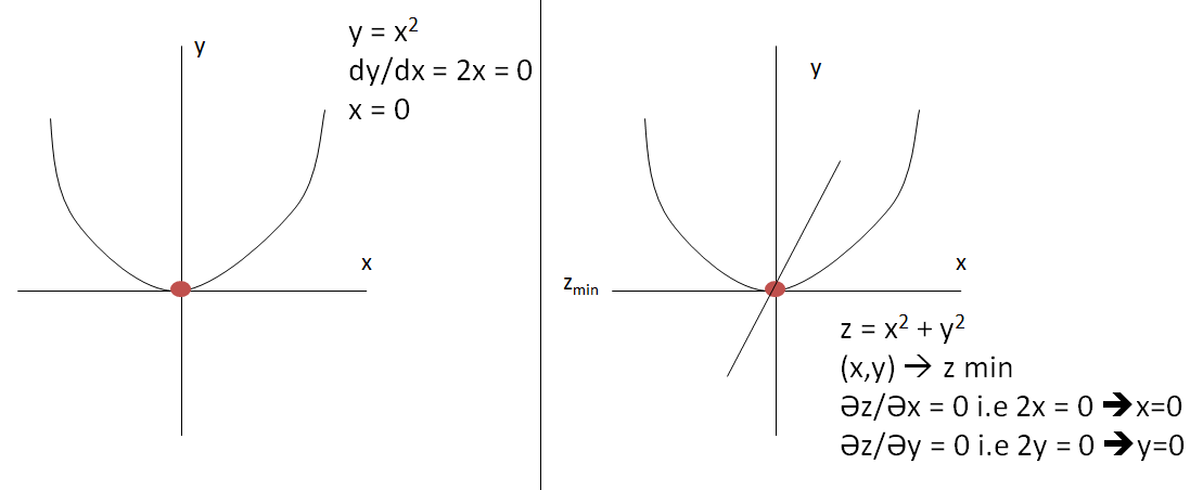
If our mathematical function depend on only one thing such y = f(x) = x2 + x, then we find derivative of y i.e dy/dx = d(fx)/dx = d(x2 + x)/dx = 2x+1
But if our mathematical function depends on two things such as z = f(x,y) = x2 + y2. therefore we will call it a partial derivative(gradient)
Then,δzδx=2x and δzδy=2y
Similarly, our loss function depends on 9 trainable parameters, hence we need to find a partial derivative of loss with respect to all trainable parameters. That is why it is called gradient (partial derivative)
Concept Of Derivative-
A derivative is the rate of change both magnitude-wise and sign-wise with respect to a variable.
dy/dx = 4, which means changing the x parameter by 1 unit will also make changes in the y parameter by 4 units.
Concept Of Minima-
Minima can be found by taking the value of the derivative equal to zero.
In image 1st we need to calculate dy/dx and assign it with zero. whatever the value of x our minima will lie on that point.
In image 2nd example for equation Z = X2 + Y2, Z will be minimum, only when the x and y both equal to 0.
Therefore, we need to find 9 derivatives by assigning them with zero with respect to loss. So that we can get minimum loss.
δLδW111,....δLδb12=0
BackPropagation Intuition-
Wnew = Wold - ηδLδW, as η=1
therefore, Wnew = Wold - δLδW
we need to repeat the below step 9 times(i.e 6 Weight and 3 Bias)
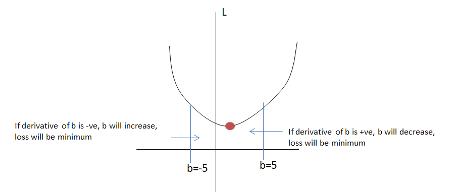
b21=b21−δLδb21
if δLδb21 (slope) is +ve then b21 will move in the negative direction and if δLδb21 (slope) is -ve then b21 will move in the positive direction. So that loss will be minimal.
Effect Of Learning Rate(η)
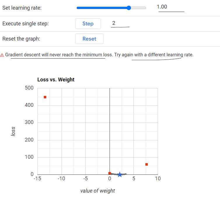
Without a learning rate, there is a high chance of parameter (W or b) to shoot out i.e. moving from +ve point to extreme negative direction OR moving from -ve point to extreme positive direction. Due to this slope will not reach a minimum and we will never get a minimum loss.
Therefore learning rate is required so that the slope will be reduced/increased slowly and reach to a minimum.
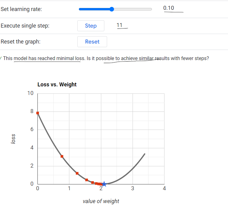
Generally Learning Rate(η) should be 0.1
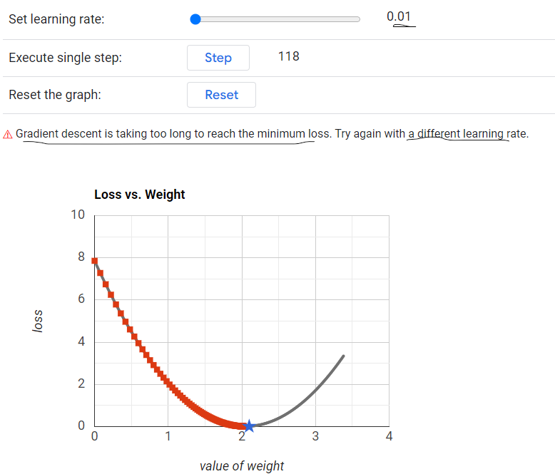
If it is very less like 0.01 then it will not converge to a minima
If it is very high like 1 then it will shoot out from a minima.
Learning Rate(η) = 0.01 - It will take too long to reach the minimum loss.
Learning Rate(η) = 0.1 - It will reach the minimum loss in fewer steps.
Learning Rate(η) = 1 - It will never reach the minimum loss.
What is Convergence?
Convergence refers to the stable point found at the end of a sequence of solutions via an iterative optimization algorithm.