Deep Learning - ANN - Artificial Neural Network - Early Stopping, Dropout. Weight Decay Tutorial
Early Stopping in Neural Networks
In machine learning, early stopping is a form of regularization used to avoid overfitting when training a learner with an iterative method, such as gradient descent. Such methods update the learner so as to make it better fit the training data with each iteration.
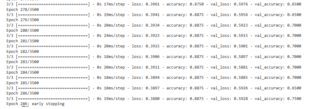
With an early stopping the model training will automatically stop at a specific epoch, once the overfitting takes place
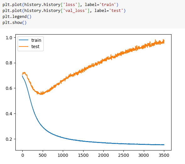
Without Early Stopping -

At some point we can check loss of test data(orange curve) is reducing until 300, then after this, it starts increasing which means it started overfitting.
So to get minimum loss or avoid overfitting we need to stop the epoch at 300 in the below plot which can be achieved by the concept of early stopping.
Using Early Stopping it stopped around 300 for the same plot-


Dropout Layer in Deep Learning | Dropout in ANN – by Nitish Srivastava
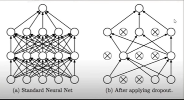
Dropout regularization is a technique to prevent neural networks from overfitting. Dropout works by randomly disabling neurons and their corresponding connections. This prevents the network from relying too much on single neurons and forces all neurons to learn to generalize better.
Why Do We Need Dropout
Deep neural networks are arguably the most powerful machine learning models available to us today. Due to a large number of parameters, they can learn extremely complex functions. But this also makes them very prone to overfitting the training data.
A possible solution to reduce overfitting is to add more data, reduce complexity, early stopping, Regularization(L1 & L2), and Dropout.
Compared to other regularization methods such as weight decay, or early stopping, dropout also makes the network more robust. This is because when applying dropout, you are removing different neurons on every pass through the network. Thus, you are actually training multiple networks with different compositions of neurons and averaging their results.
Different composition means, in dropout, we drop the random node in the input and hidden layer for a different number of epochs, so we can create randomness for each no. of epoch.
Hence, in dropout, we are training the same data with different compositions on different no. of epoch to improve neural network performance.

Random Forest Analogy
In Random Forest you are training multiple decision trees using column sampling or row sampling to create randomness i.e. ensemble learning, and at last result is based on averaging or voting from all decision trees.
Similarly, in dropout, you are training a dataset with different neural networks to create randomness and at last, averaging their results.
Both techniques are used to overcome the challenge of overfitting.
At training time weight between nodes is w and the dropout level p is 0.25, because in training time only we drop nodes. But in testing time all nodes are present, hence we need to perform some calculations on weights-
Then at testing time weight between nodes will be w(1-p) i.e. 0.75w.
Dropout Classification Practical
Code-

Dropout(0.2) – which means a drop of 2% of nodes from the hidden layer of 128 nodes, after dropout remaining node is 98% i.e 125 nodes.
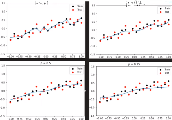
Effect of p

When the dropout value is 0(i.e. P = 0), the line is not so smooth i.e. Overfitting
When it got increased from 0.2 to 0.5 and 0.75. It got so smooth i.e. Underfitting