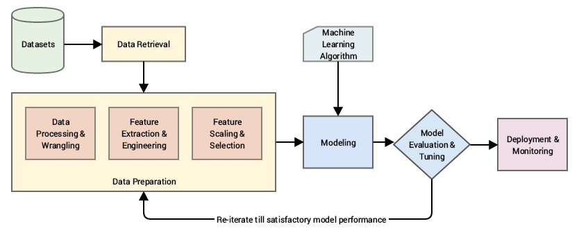
Machine Learning - Machine Learning Development Life Cycle - Feature Engineering Tutorial

Feature Engineering is the process of using domain knowledge to extract features from raw data. These features can be used to improve performance of machine learning algorithm.

 

Feature Engineering

1. Feature Transformation

• Handling Missing Data

• Handling Categorical Features
• Outlier Detection
• Feature Scaling

2. Feature Construction

• Feature Spitting

 

3. Feature Selection

• Forward Selection
• Backward Selection

4. Feature Extraction

 

Feature Engineering

1. Feature Transformation

Feature transformation is a mathematical transformation in which we apply a mathematical formula to a particular column (feature) and transform the values, which are useful for our further analysis. It is a technique by which we can boost our model performance.

• Handling Missing Data

Missing values can affect model performance, also the sci-kit learn library will not accept missing values for computation. In this case either you need to remove the missing value or fill it will any other value e.g. mean, mode, median, etc.

MCAR –Missing completely at random

 

We will remove a row if the missing row percentage is less than 5% using CCA

How to fill in the missing value?

Using univariate and multivariate-

Univariate – if you take the help of the other value in the same column to fill na, then it is univariate imputation. It is done using mean, median, and mode.

If there is an outlier, you can fill it with the median, if no outlier then fill it with the mean. If categorical value then use mode

Multivariate – If there are 4 columns, and to fill the 'na' value of column 2 you are taking the help of 1,3, and 4^th columns. Then it is multivariate. It is done using KNN, iterative

 

Arbitrary Value Imputation –  changing the value of NA into missing in case of categorical, or -1 in case of numerical. It is used when data is not missing at random.

 

Handling categorical Missing Data

Using mode or replacing the 'na' value with missing(Arbitrary value imputation)

 

Random Value Imputation

Filling the missing value with a random number from the dataset column

 

Solution To Handle Missing Data-

1] To remove them (remove row or column)

2] Missing Value Imputation(Univariate & Multivariate)

 

1] To remove them (remove row or column)

Complete Case Analysis is also called list-wise deletion of the case (for example deleting a row which has missing value). 

Complete Case Analysis means literally analyzing only those observations for which there is information in all of the variables in the dataset – used only when Missing Completely at random, missing data<5%

Isnull() & Dropna()

2] Impute Them(Univariate & Multivariate)

In simple, we can also use fillna()

Univariate Imputation– filling missing values with mean, median, and mode with the help of the same column 

Multivariate Imputation– filling missing values with the help of other multiple columns using KNN, Iterative

Mean/Median Imputation, median- mostly used for outlier data

Arbitrary Value Imputation ( used only when Data not missing completely at random)

Replacing categorical Missing value(NaN value) with a word missing

Replacing numerical Missing value with 0,99,-1 to create a difference

 

End Of Distribution Imputation

In this missing value is replaced with the end value(i.e if the column is normally distributed, then we use mean +3sigma or mean-3sigma, i.e replacing it with outlier)

If a column is skewed, then we are replacing it with IQR proximity(I.e Q1-1.5IQR or Q3+1.5IQR)

 

Handling Categorical Missing Data (MCAR)

Replacing with Most Frequent Value i.e mode

 

Random Imputation

Replacing missing values with random numbers or categories from data.

If in production. Due to random, if both users are given the same input(e.g. Fare), then both will get different outputs (i.e. age) because every time it takes a random number.

To avoid this use random_state= Fare

 

Missing Indicator 

Making separate indicator columns for missing values (True for missing values, False for non-missing)

 

Or you can also use add_indicator=True in simple imputer without using Missing Indicator.

 

Automatically Select Value for imputation

Using GridSearchCV

 

KNN Imputer (Multivariate Imputation technique)

 

Filling missing value in one row with the most similar row value. It uses euclidean distance to measure the similarity between two rows.

In KNN, k is the no. of neighbor, if k=3, then the missing value will be the average of 3 nearest neighbor value.

For example-

Step 1] Find the nearest neighbor

Suppose we have to find 2^nd row, 1^st column value.

Then we have to find the k nearest neighbor(k=2) using the Euclidian formula-

On calculating, we are able to find row 4 and row 3 are 2 nearest neighbors of row 2^nd.

Hence to find row 2^nd, column 1^st value we will do the average of rows 3 and 4, 1^st column

i.e (23+40)/2 = 31.5

 

Advantage-More accurate

Disadvantage- More no. of calculation

 

 

Multiple Imputation by chained Equations – MICE  (Iterative Imputer)

 

Use only when MCAR(missing completely at random), MAR(missing at random), MNAR(missing not at random)

 

Iteration 0

Step 1 – Fill all the NaN values with a mean of respective cols. For example, if there is 3 column(col1, col2, col3) having missing value, fill them with mean.

 

Iteration 1

Step 2 – Remove all col1 missing values, and predict the missing value of col1 using other cols (col2 & col3).

Step3 – Repeat Same Step2 for col2 and col3

Step4 – Perform subtraction i.e Iteration 1 – Iteration 0

 

Make nan value in col1 and  Perform Step 2, Step 3, till Step 4 becomes 0

 

Advantage-

Accurate

 

Disadvantage-

Slow

 

• Handling Categorical Features

The machine can only understand the numerical value. Hence, categorical value needs to be transformed into numeric, using one hot encoder, label encoder, ordinal encoder etc.

 

Two Types of Categorical Data. i.e Nominal And Ordinal.

Nominal data doesn’t have order. E.g name of the state, i.e Maharashtra, Gujarat, TamilNadu

Ordinal data have an order. E.g Class of degree i.e 1^st class > 2^nd class > 3^rd class OR excellent > good > bad

 

Encoding Categorical Data-

 

1. Ordinal Encoding (for ordinal data)

Ordinal encoding converts each label into integer values and the encoded data represents the sequence of labels

For example, suppose the company wants to recruit a person with the highest qualification. Then they will give priority to persons with PG qualification more, then UG, and last will be high school.

Which means PG > UG  > High School. 

So, in this case, we can encode qualification with the number

 i.e PG= 2, UG = 1, High School = 0 

 

 

2. Label encoding (mostly used for target variable)

Label Encoding is a popular encoding technique for handling categorical variables. In this technique, each label is assigned a unique integer based on alphabetical ordering.

It is similar to the ordinal encoder, but here order is alphabetical. 

Many of them use it on any input nominal categorical value, but as per the sci-kit-learn document it should be only used on the target column.

For example- SMS classifier target column (spam or not spam), Placement target column (placed or not placed)

 

3. One Hot Encoding (for nominal data)

One-Hot Encoding is another popular technique for treating nominal categorical variables. It simply creates additional features based on the number of unique values in the categorical feature. Every unique value in the category will be added as a feature. In this encoding technique, each category is represented as a one-hot vector.

OHE is used, so all the features have equal weight instead of ordinal.

 

 

For example, there are multiple nominal categories, such as multiple color names yellow, red, green, blue, etc. Then for all different colors, different features need to be created.

Suppose there is 50 different nominal category, then 50 different feature need to be created.

Another solution that can be used is, suppose there is 600 category, then we can use the most frequent category only, let it be the top 50, the remaining 550 categories will be named as a feature – “Other”. Therefore, the total feature will get created as 51 new features.

 

Dummy Variable Trap – It is a process of removing one (1^st) column from the n column. So, for the n nominal category, there will be a total n-1 feature. It is done to reduce multicollinearity. In simple, if the n-1 column is all 0, then obviously it will represent the 1^st column.

 

While Data Analysis, we will use pandas.get_dummies function, but while machine learning, we will not use get_dummies, instead, we will use Scikit-Learn OneHotEncoder Class.

The reason we will not use get_dummies is that get_dummies will not remember the position of the column. Every time it will generate different results.

 

Pandas.get_dummies()

 

 

 

OneHotEncoding using Sklearn

Use drop=’first’ to drop the 1^st column ( or use a dummy variable trap) from both the fuel and owner columns.

Use sparse = False, so that it will return an array, otherwise, it will return a sparse matrix (by default it is True)

Use handle_unknown = ‘ ignore’ . In the future when an unknown category is encountered during transform, the resulting one-hot encoded columns for this feature will be all zeros. In the inverse transform, an unknown category will be denoted as None.

By default, it is an ‘error’ that will Raise an error if an unknown category is present during the transform.

 

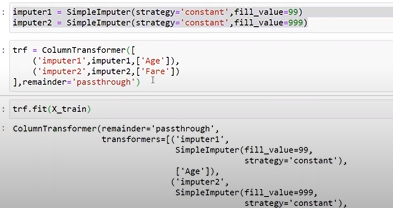
It is hectic to process to attach the above array with the remaining column brands and km_driven

So, in this case, we will use a column transformer, where we can apply different transformations to multiple columns at a time in one line

• Outlier Detection

 

What are outliers?

An outlier is an abnormal value (It is at an abnormal distance from the rest of the data points).

 

When is outlier dangerous? 

Outliers in the dataset will affect the statistical result or provide incorrect results. Hence, outliers need to be removed, after outlier detection 

Sometimes it is not dangerous, for example, anomaly detection like credit card fraud, here it can be useful.

 

Effect Of outlier on ML Algorithms

Weight-based algorithm - Linear, logistic, AdaBoost, and deep learning are affected more by outliers.

While tree based algorithm has no effect on outliers.

 

How to treat outliers?

Trimming – remove outlier

Capping – i.e. by applying a limit, for example, age should be limited to 18-60, If age is 80, then it will be capped to max value. i.e 60.

Missing Value –treat the outlier as a missing value

Discretization – Range the value. e.g. 10-20,20-30, 90-100. So. Here 100 value is considered to be in the range of 90.

 

How to detect outliers?

 1] Using Normal Distribution (Z-Score)

If your value lies out of range (mean - 3 sigmas, mean + 3 sigmas) is considered an outlier

 

2] Skewed Distribution (using IQR)

If your value lies out of range (Q1 – 1.5 IQR, Q3 + 1.5 IQR)  is considered as outlier

 

3] Other Distribution (percentile-based approach)

 

Other normal visualization techniques- 

4] simply sort your data

5] Graph your data using boxplots, histograms, and scatterplots.

 

1] Using Normal Distribution (Z-Score)

Maximum value lies between (mean + sigma, mean + sigma) i.e 68.4%

Between (mean - 2 sigma, mean + 2 sigma) 95.4% value lies

Between (mean - 3 sigma, mean + 3 sigma) 99.7% value lies

 

If your value lies out of range (mean - 3 sigmas, mean + 3 sigmas). i.e. remaining 0.3% will be considered Outlier.

It is similar to calculating the z-score-

rule of thumb is if Z-Score for a specific data point is less than -3 or greater than 3 is a suspected outlier.

 

Outlier Treatment using Trimming(remove outlier value) And Capping.

 

2] Skewed Distribution (using IQR)

If your value lies out of range (Q1 – 1.5 IQR, Q3 + 1.5 IQR)

IQR = Q3 – Q1

Q2 – Median

 

You can check skewness using .skew(), if the value is greater than 0.5 right skewed,0- normal distribution, -0.5  - left skewed.

IQR is calculated using percentile(quantile) i.e percentile75-percentile25

 

3] Other Distribution (percentile-based approach)

Max value – 100 Percentile, Min Value – 0 Percentile

50 Percentile – Median

Take any same percentile value for both ends to be considered as an outlier. Let's take 2.5% 

Then the value lies out of range (2.5%, 97.5%) will be considered an outlier

Whenever you are using the percentile method with capping, is known as Winserization.

 

• Feature Scaling

Feature scaling refers to the process of scaling the value of a numerical feature into a fixed range using standardization or normalization.

 

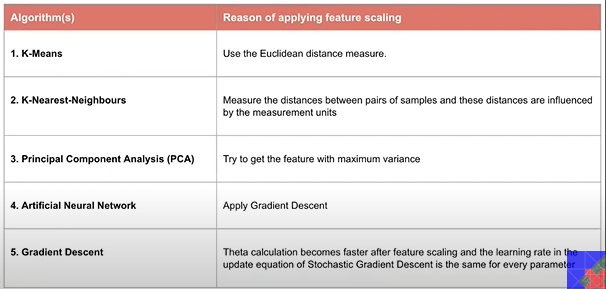
Why do we need feature scaling?

Feature scaling is important because when training the model, some features will get dominated by the other feature.

In the below example, the salary column will dominate the age column, due to the large difference in their value. To prevent this we use the feature scaling technique.

 

 

Certain ways to perform feature scaling-

 

1. Standard Scaler

StandardScaler is used to resize the distribution of values ​​so that the mean of the observed values ​​is 0, which means it produces a distribution centered at 0 and the standard deviation is 1.

µ is the mean, σ is the standard deviation.

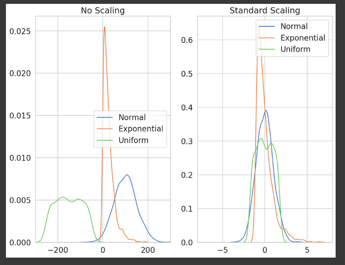
The resulting distributions overlap heavily. And the feature will become normally distributed.

Disadvantage - Not robust to outliers therefore shape become much narrower.

 

 

Decision tree, Random Forest, XGBoost, and Gradient Boost doesn’t have effect of scaling.

 

When to use standardization?

 

Note- In standard scalar, first mean centering will be done so that the mean becomes 0, and then standardization on the basis of standard deviation is done. As the standard deviation increase dataset will more get squeezed to the center.

 

2. MinMaxScaler

 

It scales each variable/feature in the [0,1] range. If it contains a negative value, then it scales each variable/feature in the [-1,1] range.

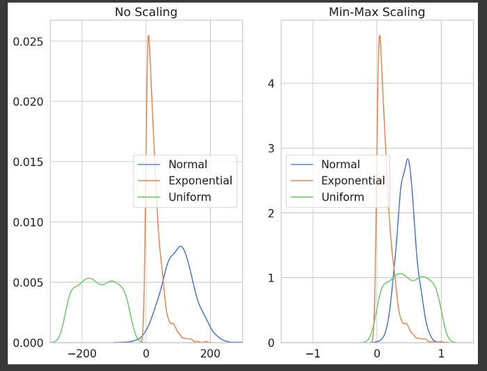
MinMaxScaler

 

3. Robust Scaling

 

Robust Scaler algorithms scale features that are robust to outliers. The method it follows is almost similar to the MinMax Scaler but it uses the interquartile range (rather than the min-max used in MinMax Scaler). The median and scales of the data are removed by this scaling algorithm according to the quantile range.

Where Q1 is the 1st quartile, and Q3 is the third quartile.

Min-Max scaler brought the outliers close to it in the range of [0,1] whereas the Robust Scaler scaled the data down and also maintained the distance proportion with outliers.

4. Mean Normalization

It is similar to the min-max scaler, instead of subtracting min from the numerator, it will subtract the mean. So that dataset becomes mean centering. Its values ranges between -1 to +1.

5. MaxaAbsScaling

An estimator that scales the input values so that the maximum absolute value is 1.0.

X_i^’ = X_i/|X_max|

Useful when there is sparse data.

 

class sklearn.preprocessing.MaxAbsScaler(*, copy=True)

 

Why does fit need to be applied to the training dataset and transformed on both the train and test datasets?

https://towardsdatascience.com/what-and-why-behind-fit-transform-vs-transform-in-scikit-learn-78f915cf96fe#:~:text=fit_transform()%20is%20used%20on,to%20scale%20our%20test%20data. 

 

2. Feature Construction

Feature construction is a process that discovers missing information by splitting the original feature into a new additional feature for better results.

Feature construction attempts to increase the expressive power of the original features. Usu ally the dimensionality of the new feature set is expanded and is bigger than that of the original feature set.

For example creating a new extra feature such as City, State, or Pincode by splitting the original feature address which is also known as Feature Spitting

 

Learn the Curse Of Dimensionality before learning feature selection and feature extraction

• Curse Of Dimensionality

Column=features=Dimensionaltiy

The curse of Dimensionality refers to a set of problems that arise when working with high-dimensional data. The dimension of a dataset corresponds to the number of attributes/features that exist in a dataset. A dataset with a large number of attributes, generally of the order of a hundred or more, is referred to as high dimensional data. Some of the difficulties that come with high dimensional data is analyzing or visualizing the data to identify patterns, and some while training machine learning models. The difficulties related to training machine learning models due to high dimensional data are referred to as the ‘Curse of Dimensionality’.

Example – Digit (images) using optimum feature, instead of all columns (28 x 28 =784). i.e. column more than required will increase sparsity.

Problem-

• Performance decreases
• Computation increase

Solution-

• Dimensionality Reduction

feature selection & feature extraction

Dimensionality Reduction is the process of reducing the number of input variables in a dataset, also known as the process of converting the high-dimensional variables into lower-dimensional variables without changing their attributes of the same.

 

3. Feature Selection

Feature Selection is the method of reducing the input variable to your model by using only relevant data and getting rid of noise in data.

For example- in mnist data, we can use only important features instead of all feature

In the above image, the green part is an important feature. And red part is an unimportant feature

• Forward Selection
• Backward Elimination

4. Feature Extraction

Feature Extraction is a process to create/extract new intermediate features from the original feature in a dataset. 

For example creating a completely new feature total area from the multiple original features such as bathroom area, hall area, kitchen area, and bedroom area.

• PCA
• LDA
• TSNE

 

Difference between feature construction and feature extraction -

Feature construction often expands the feature space, whereas feature extraction usually reduces the feature space.