Machine Learning - Ensemble Learning - Boosting Tutorial

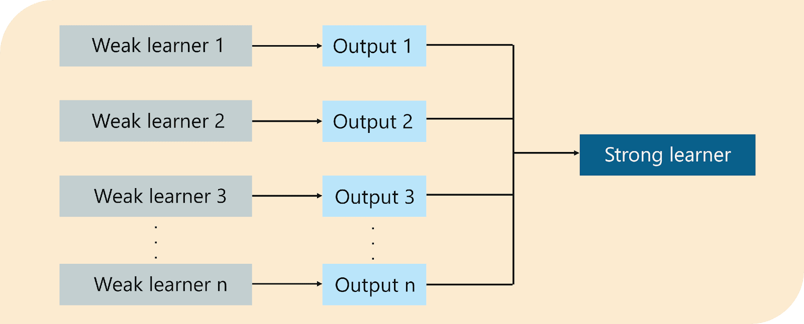
Boosting is an ensemble learning technique that uses a set of Machine Learning algorithms to convert weak learner (model with low accuracy) to strong learners (model with high accuracy)  in order to increase the accuracy of the model. 

In this a model is built from the training data. Then the second model is built which tries to correct the errors present in the first model. This procedure is continued and models are added until either the complete training data set is predicted correctly or the maximum number of models are added.

Decision Stump - The Decision Stump is used for generating a decision tree with only one single split or a decision tree with maximum depth one.

• AdaBoost – Stagewise Additive method

Adaptive boosting or AdaBoost usually use decision trees for modelling. AdaBoost initially gives the same weight to each dataset. Then, it automatically adjusts the weights of the data points after every decision tree. It gives more weight to incorrectly classified items to correct them for the next round. It repeats the process until the residual error, or the difference between actual and predicted values, falls below an acceptable threshold.

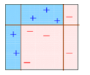
This diagram explains Ada-boost. Let’s understand it closely:

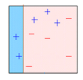
Box 1: You can see that we have assigned equal weights to each data point and applied a decision stump to classify them as + (plus) or – (minus). The decision stump (D1) has generated vertical line at left side to classify the data points. We see that, this vertical line has incorrectly predicted three + (plus) as – (minus). In such case, we’ll assign higher weights to these three + (plus) and apply another decision stump.

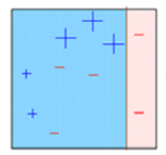
Box 2: Here, you can see that the size of three incorrectly predicted + (plus) is bigger as compared to rest of the data points. In this case, the second decision stump (D2) will try to predict them correctly. Now, a vertical line (D2) at right side of this box has classified three mis-classified + (plus) correctly. But again, it has caused mis-classification errors. This time with three -(minus). Again, we will assign higher weight to three – (minus) and apply another decision stump.

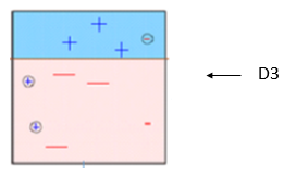
Box 3: Here, three – (minus) are given higher weights. A decision stump (D3) is applied to predict these mis-classified observation correctly. This time a horizontal line is generated to classify + (plus) and – (minus) based on higher weight of mis-classified observation.

Box 4: Here, we have combined D1, D2 and D3 to form a strong prediction having complex rule as compared to individual weak learner. You can see that this algorithm has classified these observation quite well as compared to any of individual weak learner.

For adaboost example or How to calculate alpha or weight? See video – 99 & 100th-

Bagging Vs Boosting

1] Type Of Model used – 

In bagging we used model, which has low bias high variance such as Fully grown decision tree, SVM, KNN

In boosting we used model, which has high bias low variance such as shallow decision tree(e.g decision stump, having depth 1), linear regression, logistic regression.

2] Sequential Vs Parallel

In bagging, model is trained parallel, while in boosting, model is trained sequentially.

3] Weightage of base learner

In bagging, each base model has equal weight, while in boosting, model can have different weight

• Gradient Boosting

Gradient Boosting is similar to AdaBoost. the only difference between AdaBoost and Gradient Boosting is that Gradient Boosting does not give incorrectly classified items more weight. 

Instead, Gradient Boosting minimize the loss function by using stagewise additive modelling technique. It will minimize gross prediction error if combined with the previous set of model. so that the present base model is always more effective than the previous one. 

This method attempts to generate accurate results initially instead of correcting errors throughout the process, like AdaBoost. 

When the target column is continuous we use Gradient Boosting Regressor, whereas when it is classification problem, we use Gradient Boosting Classifier. Only difference between two is loss function.

For this reason, Gradient Boosting can lead to more accurate results. Gradient Boosting can help with both classification and regression-based problems.

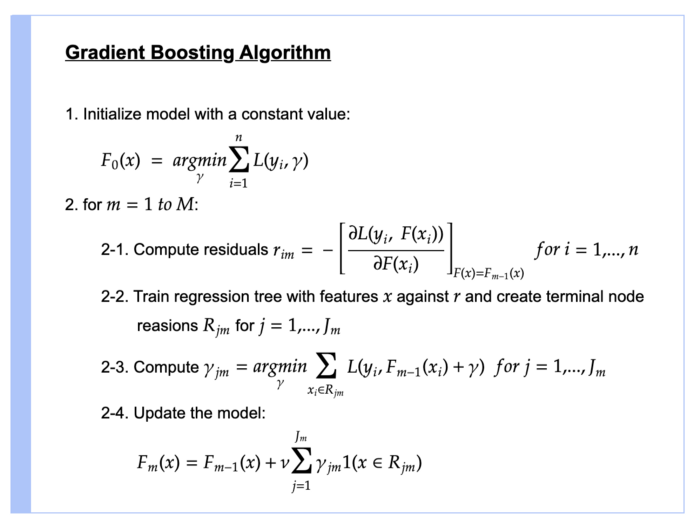
Algorithm-

R&D Spend, Administration and  Marketing Spend is input column, profit is output column

Step 1] In this find the mean of output/target column(target) and initialize means as f0(x)

Step 2] 

2-1] In this find the residual by subtracting f0(x) from profit and initialize it with ri1

2-2] Train the decision tree with R&D Spend, Administration and Marketing Spend as input column and ri1 as output column.

We have use max depth =1 for the decision tree, since our dataset is small. For depth 1, there will be two terminal node. i.e R₁₁ and R₂₁, where R₁₁ is 1^st terminal region of 1^st decision tree and R₂₁ is 2^nd terminal region of 1^st decision tree.

2-3] In this we need to find gamma for R₁₁ and R₂₁, on computing that equation we get

Y_i – f0(x) – gamma = 0

Gamma₁₁ = 91 -142.33 = -51.33

Y_i – f0(x₁) – gamma + Y₂ – f0(x₁) – gamma = 0

192 – 142 – gamma – 144 – 142 – gamma = 0

Gamma₁₁ = 25.66

It is same ri1, because we use loss function as least square mean, if we use other loss function, then answer will be different. So, it is just coincidence. Both have no relation.

2-4]  In this step we are performing stagewise additive 

Suppose m = 4, hereDT₄ is output of decision tree 4.

Then f4(x) = f3(x) + DT₄

But f3(x) = f2(x) + DT₃, f2(x) = f1(x) + DT₂, f1(x) = f0(x) + DT₁ , all are in recursive form

On combining all , we get f4(x) = f0(x) + DT₁ + DT₂ + DT₃ + DT₄

Hence, final result will be f_m(x) or f(x)

Ada Boost VS Gradient Boost

1] In ada boost we use decision stump(decision tree with max depth 1), and in gradient boost we use decision tree with max leaf node is between 8 to 32

2] In ada boost we give weight to each model, while in gradient boost we use learning rate, which is same for all model.

• Xtreme Gradient Boosting

Extreme Gradient Boosting (XGBoost) improves gradient boosting for computational speed and scale in several ways. XGBoost uses multiple cores on the CPU so that learning can occur in parallel during training. It is a boosting algorithm that can handle extensive datasets, making it attractive for big data applications. The key features of XGBoost are parallelization, distributed computing, cache optimization, and out-of-core processing.

Algorithms based on Bagging and Boosting
4.1 Bagging meta-estimator
4.2 Random Forest

4.6 Light GBM